前几天写了学习Embeddings的例子,因为琢磨了各个细节,自己也觉得受益匪浅。于是,开始写下一个LSTM的教程吧。
还是Udacity上那个课程。
RNN是一个非常棒的技术,可能它已经向我们揭示了“活”的意义。RNN我已经尝试学习了几次,包括前面我这篇笔记,所以就直接进入代码阅读吧。
读例子程序:
1. 引入库文件
# These are all the modules we'll be using later. Make sure you can import them
# before proceeding further.
from __future__ import print_function
import os
import numpy as np
import random
import string
import tensorflow as tf
import zipfile
from six.moves import range
from six.moves.urllib.request import urlretrieve
2. 下载数据
然后下载数据,如果前面已经下载过,那直接把text8.zip拷过来就可以用。
url = 'http://mattmahoney.net/dc/'

def maybe_download(filename, expected_bytes):
  """Download a file if not present, and make sure it's the right size."""
  if not os.path.exists(filename):
    filename, _ = urlretrieve(url + filename, filename)
  statinfo = os.stat(filename)
  if statinfo.st_size == expected_bytes:
    print('Found and verified %s' % filename)
  else:
    print(statinfo.st_size)
    raise Exception(
      'Failed to verify ' + filename + '. Can you get to it with a browser?')
  return filename

filename = maybe_download('text8.zip', 31344016)
3. 读入文本
读文件稍微有些不一样,不是处理成list,而是直接读成一个字符串,因为后面用到的就是串数据。
def read_data(filename):
  f = zipfile.ZipFile(filename)
  for name in f.namelist():
    return tf.compat.as_str(f.read(name))
  f.close()

text = read_data(filename)
print('Data size %d' % len(text))
4. 生成训练数据集函数
切割一下,留1000个字符做检验,其他99999000个字符拿来训练。
valid_size = 1000
valid_text = text[:valid_size]
train_text = text[valid_size:]
train_size = len(train_text)
print(train_size, train_text[:64])
print(valid_size, valid_text[:64])
5. 两个工具函数
建立两个函数char2id和id2char,用来把字符对应成数字。
本程序只考虑26个字母外加1个空格字符,其他字符都当做空格来对待。所以可以用两个函数,通过ascii码加减,直接算出对应的数值或字符。
vocabulary_size = len(string.ascii_lowercase) + 1 # [a-z] + ' '
first_letter = ord(string.ascii_lowercase[0])

def char2id(char):
  if char in string.ascii_lowercase:
    return ord(char) - first_letter + 1
  elif char == ' ':
    return 0
  else:
    print('Unexpected character: %s' % char)
    return 0

def id2char(dictid):
  if dictid > 0:
    return chr(dictid + first_letter - 1)
  else:
    return ' '

print(char2id('a'), char2id('z'), char2id(' '), char2id('ï'))
print(id2char(1), id2char(26), id2char(0))
6. 生成训练数据集函数
这次 BatchGenerator 做的比前两天的那个要认真了,用了成员变量来记录位置,而不是用全局变量。
用 BatchGenerator.next() 方法,可以获取一批子字符串用于训练。
batch_size 是每批几串字符串,num_unrollings 是每串子字符串的长度(实际上字符串开头还加了上一次获取的最后一个字符,所以实际上字符串长度要比 num_unrollings 多一个)。
batch_size=64
num_unrollings=10

class BatchGenerator(object):
  def __init__(self, text, batch_size, num_unrollings):
    self._text = text
    self._text_size = len(text)
    self._batch_size = batch_size
    self._num_unrollings = num_unrollings
    segment = self._text_size // batch_size
    self._cursor = [ offset * segment for offset in range(batch_size)]
    self._last_batch = self._next_batch()

  def _next_batch(self):
    """Generate a single batch from the current cursor position in the data."""
    batch = np.zeros(shape=(self._batch_size, vocabulary_size), dtype=np.float)
    for b in range(self._batch_size):
      batch[b, char2id(self._text[self._cursor[b]])] = 1.0
      self._cursor[b] = (self._cursor[b] + 1) % self._text_size
    return batch

  def next(self):
    """Generate the next array of batches from the data. The array consists of
    the last batch of the previous array, followed by num_unrollings new ones.
    """
    batches = [self._last_batch]
    for step in range(self._num_unrollings):
      batches.append(self._next_batch())
    self._last_batch = batches[-1]
    return batches
真不愧是优秀程序员写的代码,这个函数写的又让我学习了!
它在初始化的时候先根据 batch_size 把段分好,然后设立一组游标 _cursor ,是一组哦,不是一个哦!然后定义好 _last_batch 看或许到哪了。
然后获取需要的字符串的时候,是一批一批的获取各个字符。
这样做,就可以针对整段字符串均匀的取样,从而避免某些地方学的太细,某些地方又没有学到。
值得注意的是,在RNN准备数据的时候,所喂数据的结构是很容易搞错的。在前面博客中,也有很多同学对于他使用 transpose 的意义没法理解。这里需要详细记录一下。
BatchGenerator.next() 返回的数据格式,是一个list,list的长度是 num_unrollings+1,每一个元素,都是一个(batch_size,27)的array,27是 vocabulary_size,一个27维向量代表一个字符,是one-hot encoding的格式。
所以,喂这一批数据进神经网络的时候,理论上是先进去一批的首字符,然后再进去同一批的第二个字符,然后再进去同一批的第三个字符…
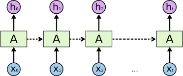
也就是说,下图才是真正的RNN的结构,我们要做的,是按照顺序一个一个的按顺序把东西喂进去。这个图,我看到名字叫 RNN-rolled:
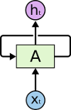
我们平时看到的向右一路展开的RNN其实向右方向(我用了虚线)是代表先后顺序(同时也带记忆数据流),跟上下方向意义是不一样的。有没有同学误解那么一排东西是可以同时喂进去的?这个图,我看到名字叫 RNN-unrolled。
7. 另外两个工具函数
再定义两个用来把训练数据转换成可展现字符串的函数。
characters 先从one-hot encoding变回数字,再用id2char变成字符。
batches2string 则将训练数据变成可以展现的字符串。高手这么一批一批的处理数据逻辑还这么绕,而不是按凡人逻辑一个一个的处理让我觉得有点窒息的感觉,自感智商捉急了。
def characters(probabilities):
  """Turn a 1-hot encoding or a probability distribution over the possible
  characters back into its (most likely) character representation."""
  return [id2char(c) for c in np.argmax(probabilities, 1)]

def batches2string(batches):
  """Convert a sequence of batches back into their (most likely) string
  representation."""
  s = [''] * batches[0].shape[0]
  for b in batches:
    s = [''.join(x) for x in zip(s, characters(b))]
  return s

train_batches = BatchGenerator(train_text, batch_size, num_unrollings)
valid_batches = BatchGenerator(valid_text, 1, 1)

print(batches2string(train_batches.next()))
print(batches2string(train_batches.next()))
print(batches2string(valid_batches.next()))
print(batches2string(valid_batches.next()))
8. 另外四个工具函数
四个函数,给训练中输出摘要时使用。
def logprob(predictions, labels):
  """Log-probability of the true labels in a predicted batch."""
  predictions[predictions < 1e-10] = 1e-10
  return np.sum(np.multiply(labels, -np.log(predictions))) / labels.shape[0]

def sample_distribution(distribution):
  """Sample one element from a distribution assumed to be an array of normalized
  probabilities.
  """
  r = random.uniform(0, 1)
  s = 0
  for i in range(len(distribution)):
    s += distribution[i]
    if s >= r:
      return i
  return len(distribution) - 1

def sample(prediction):
  """Turn a (column) prediction into 1-hot encoded samples."""
  p = np.zeros(shape=[1, vocabulary_size], dtype=np.float)
  p[0, sample_distribution(prediction[0])] = 1.0
  return p

def random_distribution():
  """Generate a random column of probabilities."""
  b = np.random.uniform(0.0, 1.0, size=[1, vocabulary_size])
  return b/np.sum(b, 1)[:,None]
logprob: 用来测量预测工作完成的如何。
先回忆一下 cross_entropy:
那么,
\[logprob = { Cross Entropy \over N }\]后面三个函数 sample_distribution sample random_distribution 是一起使用的。
random_distribution 就是生成一个平均分布的,加总和为 1 的 array。但是我不知道为何写的这么花哨,我试了半天,似乎 b/np.sum(b, 1)[:,None] 和 b/np.sum(b) 的意思是一样的。
sample 则是靠 sample_distribution 以传入的 prediction 的概率,随机取一个维设成 1 ,其他都设成 0 ,也就是按照 prediction 的概率获得一个随机字母。(为啥不直接取概率最大的那个字母呢?搞这么复杂真的好吗?)
9. 定义Tensorflow模型
分为几个部分:定义变量,定义LSTM Cell,定义输入接口,循环执行LSTM Cell,定义loss,定义优化,定义预测。
num_nodes 是代表这个神经网络中LSTM Cell层的Cell个数。
num_nodes = 64

graph = tf.Graph()
with graph.as_default():
1) 定义变量
  # Parameters:
  # Input gate: input, previous output, and bias.
  ix = tf.Variable(tf.truncated_normal([vocabulary_size, num_nodes], -0.1, 0.1))
  im = tf.Variable(tf.truncated_normal([num_nodes, num_nodes], -0.1, 0.1))
  ib = tf.Variable(tf.zeros([1, num_nodes]))
  # Forget gate: input, previous output, and bias.
  fx = tf.Variable(tf.truncated_normal([vocabulary_size, num_nodes], -0.1, 0.1))
  fm = tf.Variable(tf.truncated_normal([num_nodes, num_nodes], -0.1, 0.1))
  fb = tf.Variable(tf.zeros([1, num_nodes]))
  # Memory cell: input, state and bias.
  cx = tf.Variable(tf.truncated_normal([vocabulary_size, num_nodes], -0.1, 0.1))
  cm = tf.Variable(tf.truncated_normal([num_nodes, num_nodes], -0.1, 0.1))
  cb = tf.Variable(tf.zeros([1, num_nodes]))
  # Output gate: input, previous output, and bias.
  ox = tf.Variable(tf.truncated_normal([vocabulary_size, num_nodes], -0.1, 0.1))
  om = tf.Variable(tf.truncated_normal([num_nodes, num_nodes], -0.1, 0.1))
  ob = tf.Variable(tf.zeros([1, num_nodes]))
  # Variables saving state across unrollings.
  saved_output = tf.Variable(tf.zeros([batch_size, num_nodes]), trainable=False)
  saved_state = tf.Variable(tf.zeros([batch_size, num_nodes]), trainable=False)
  # Classifier weights and biases.
  w = tf.Variable(tf.truncated_normal([num_nodes, vocabulary_size], -0.1, 0.1))
  b = tf.Variable(tf.zeros([vocabulary_size]))
LSTM Cell 首先有三个门,input output forget三门。
Memory cell 暂时不知道是个什么。
saved_output 是向上的产出,saved_state 是自己的状态记忆。
w 和 b 是最后用来做一个 full connection 的标准神经网络层,把结果变为 vocabulary_size 个之一。
2) 定义LSTM Cell
  # Definition of the cell computation.
  def lstm_cell(i, o, state):
    """Create a LSTM cell. See e.g.: http://arxiv.org/pdf/1402.1128v1.pdf
    Note that in this formulation, we omit the various connections between the
    previous state and the gates."""
    input_gate = tf.sigmoid(tf.matmul(i, ix) + tf.matmul(o, im) + ib)
    forget_gate = tf.sigmoid(tf.matmul(i, fx) + tf.matmul(o, fm) + fb)
    update = tf.matmul(i, cx) + tf.matmul(o, cm) + cb
    state = forget_gate * state + input_gate * tf.tanh(update)
    output_gate = tf.sigmoid(tf.matmul(i, ox) + tf.matmul(o, om) + ob)
    return output_gate * tf.tanh(state), state
这里定义的 LSTM Cell 似乎并不是我们平时熟悉的那种,而是如下图(http://arxiv.org/pdf/1402.1128v1.pdf):
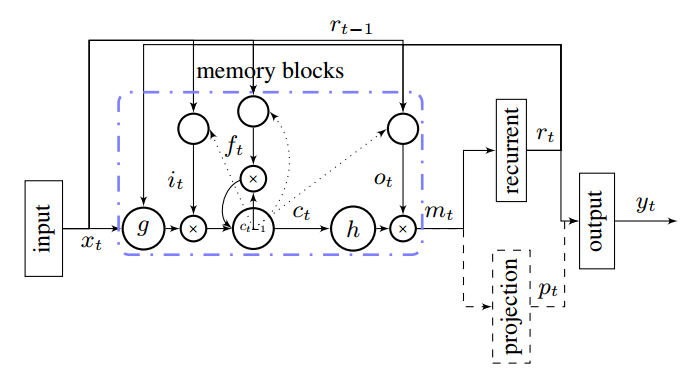
初看这个图可能不是很能理解,于是我重新画了一下:
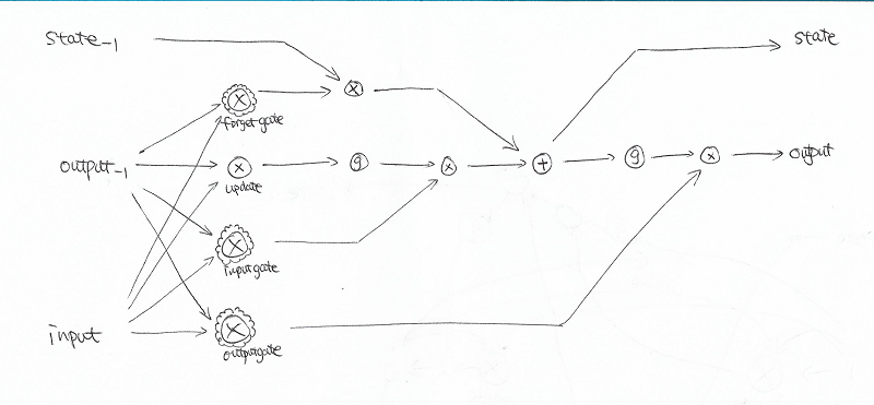
我手画的图例解释:
(1) \(\otimes\)代表两个数据源乘上参数后相加。\(\oplus\)代表两个数据源相加。
(2) \(\otimes\)外面再加花边的,代表两个数据源相乘后再取 sigmoid 。
(3) 圆圈里是 \(g\) 的,代表取 tanh 。
(4) \(State_{-1}\) 下标-1代表这是上一次迭代时的结果。
回想一下,
sigmoid函数产生一个(0,1)的数,tanh函数产生一个(-1,1)的数。
作为对比,我再引用一个我认为画的最完美的标准 LSTM Cell 图,来自 Colah 的博客:
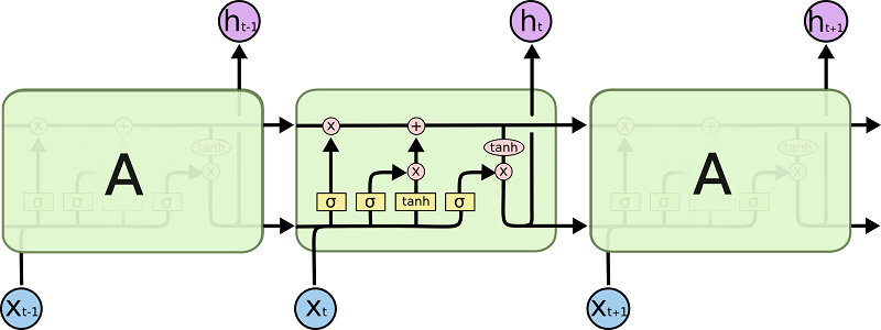
Colah 图例解释:
(1) 方形中带 \(\sigma\) ,代表两个数据源连接在一起后乘参数,再取 sigmoid 。(嗯,这里有不同:Colah 博客中标准的 LSTM Cell 中,这里的操作是先接在一起,再乘参数,而我们这里是先各自乘参数,再相加。)
(2) 方形中带 \(tanh\) ,代表两个数据源连接在一起后乘参数,再取 tanh 。(这里也是)
(3) 椭圆形中带 \(tanh\), 代表直接取 tanh 。
(4) \(\otimes\)代表两个数据源相乘。\(\oplus\)代表两个数据源相加。
(5) 两条从过去\(-1\)到当前 Cell 再到未来\(+1\)的横向黑色线条箭头,上方代表 state,下方代表 output。
所以像论文里指出的,这里实现的 LSTM Cell 含有更多参数,效果更好?这种比较目前超出我的认知范围,以后再细看。
3) 定义输入接口
  # Input data.
  train_data = list()
  for _ in range(num_unrollings + 1):
    train_data.append(
      tf.placeholder(tf.float32, shape=[batch_size,vocabulary_size]))
  train_inputs = train_data[:num_unrollings]
  train_labels = train_data[1:]  # labels are inputs shifted by one time step.
这里也是一个 batch 同时处理的。但为了容易理解,我先假设 batch_size=1 ,然后假设我们要训练一个字符串 abcdefg。
那么 train_inputs 是 abcdef,train_labels 是 bcdefg 。
4) 循环执行LSTM Cell
  # Unrolled LSTM loop.
  outputs = list()
  output = saved_output
  state = saved_state
  for i in train_inputs:
    output, state = lstm_cell(i, output, state)
    outputs.append(output)
根据前面定义变量的时候规定,初始 saved_output 和 saved_state 都是全零。
依次输入 a b c d e f ,把每一次的输出放在一起形成一个 list 就是 outputs。
5) 定义loss
  # State saving across unrollings.
  with tf.control_dependencies([saved_output.assign(output),
                                saved_state.assign(state)]):
    # Classifier.
    logits = tf.nn.xw_plus_b(tf.concat(0, outputs), w, b)
    loss = tf.reduce_mean(
      tf.nn.softmax_cross_entropy_with_logits(
        logits, tf.concat(0, train_labels)))
因为不是顺序执行语言,一般模型如果不是相关的语句,其执行是没有先后顺序的,control_dependencies 的作用就是建立先后顺序,保证前面两句被执行后,才执行后面的内容。
这里也就是先把 saved_output 和 saved_state 保存之后,再计算 logits 和 loss。否则因为下面计算时没有关联到 saved_output 和 saved_state,如果不用 control_dependencies 那上面两句保存就不会被优化语句触发。
tf.concat(0, values) 是指在 0 维上把 values 连接起来。本来 outputs 是一个 list,每一个元素都是一个27维向量表示一个字母(还是假设 batch_size=1)。
通过 tf.concat 把结果连接起来,成为一个向量,可以拿来乘以 w 加上 b 这样进入一个 full connection,从而得到 logits 。
然后再通过 softmax_cross_entropy_with_logits 比较连接并 full connection 的 outputs 和 连接起来的 train_labels ,得到 loss 。
6) 定义优化
  # Optimizer.
  global_step = tf.Variable(0)
  learning_rate = tf.train.exponential_decay(
    10.0, global_step, 5000, 0.1, staircase=True)
  optimizer = tf.train.GradientDescentOptimizer(learning_rate)
  gradients, v = zip(*optimizer.compute_gradients(loss))
  gradients, _ = tf.clip_by_global_norm(gradients, 1.25)
  optimizer = optimizer.apply_gradients(
    zip(gradients, v), global_step=global_step)
tf.train.exponential_decay 可以用来实现 learning_rate 的指数型衰减,越到后面 learning_rate 越小。(依赖后面修改 global_step 值来实现)
optimizer 定义成使用标准 Gradient Descent 。每一种 optimizer 都有几个标准接口,我们前面常用的是 minimize 接口,他自动的调整整个 Graph 中可调节的 Variables 尝试最小化 loss。其实 minimize 函数就是这两步并起来: compute_gradients 和 apply_gradients。先计算梯度值,然后再把那些参数减去梯度值。这里把两步分开了,为了在 apply 之前先处理一下梯度值,Tensorflow 给了详细解释,我们来看看[手册][manual-compute-gradients]。
compute_gradients 函数返回一个list,里面是一对一对的 gradient 和 variable,说明针对某个可调整的变量,他的梯度是多少。
clip_by_global_norm 避免梯度值过大产生 Exploding Gradients 梯度爆炸问题,视频里有这么一个图:
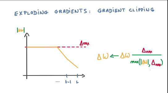
clip_by_global_norm 的具体计算是,先计算 global_norm ,也就是整个 tensor 的模(二范数)。看这个模是否大于文中的1.25,如果大于,则结果等于 gradients * 1.25 / global_norm,如果不大于,就不变。
最后,apply_gradients。这里传入的 global_step 是会被修改的,每次加一,这样下次计算 learning_rate 的时候就会使用新的 global_step 值。
7) 定义预测
  # Predictions.
  train_prediction = tf.nn.softmax(logits)

  # Sampling and validation eval: batch 1, no unrolling.
  sample_input = tf.placeholder(tf.float32, shape=[1, vocabulary_size])
  saved_sample_output = tf.Variable(tf.zeros([1, num_nodes]))
  saved_sample_state = tf.Variable(tf.zeros([1, num_nodes]))
  reset_sample_state = tf.group(
    saved_sample_output.assign(tf.zeros([1, num_nodes])),
    saved_sample_state.assign(tf.zeros([1, num_nodes])))
  sample_output, sample_state = lstm_cell(
    sample_input, saved_sample_output, saved_sample_state)
  with tf.control_dependencies([saved_sample_output.assign(sample_output),
                                saved_sample_state.assign(sample_state)]):
    sample_prediction = tf.nn.softmax(tf.nn.xw_plus_b(sample_output, w, b))
sample_input 是一个1-hot编码过的字符。
建立初始 state 和 output,经过同样的 LSTM Cell,得到下一个预测的字符 sample_prediction。
10. 开始训练
1) 训练
注意到这里喂进去的字符串长度正好是 num_unrollings + 1,恰好对应前面 BatchGenerator.next() 获取的时候得到的字符串长度,也恰好对应了模型定义里 train_inputs 和 train_labels 错开1个字符。
mean_loss 用来加总各步的 loss 值,用来后面输出。(还是建议叫 subtotal_loss)
num_steps = 7001
summary_frequency = 100

with tf.Session(graph=graph) as session:
  tf.initialize_all_variables().run()
  print('Initialized')
  mean_loss = 0
  for step in range(num_steps):
    batches = train_batches.next()
    feed_dict = dict()
    for i in range(num_unrollings + 1):
      feed_dict[train_data[i]] = batches[i]
    _, l, predictions, lr = session.run(
      [optimizer, loss, train_prediction, learning_rate], feed_dict=feed_dict)
    mean_loss += l
2) 定期输出摘要
他怎么不用 tensorflow 来计算呀,反而用 numpy 来计算,很奇怪。来仔细看看。
    if step % summary_frequency == 0:
      if step > 0:
        mean_loss = mean_loss / summary_frequency
      # The mean loss is an estimate of the loss over the last few batches.
      print(
        'Average loss at step %d: %f learning rate: %f' % (step, mean_loss, lr))
      mean_loss = 0
      labels = np.concatenate(list(batches)[1:])
      print('Minibatch perplexity: %.2f' % float(
        np.exp(logprob(predictions, labels))))
      if step % (summary_frequency * 10) == 0:
        # Generate some samples.
        print('=' * 80)
        for _ in range(5):
          feed = sample(random_distribution())
          sentence = characters(feed)[0]
          reset_sample_state.run()
          for _ in range(79):
            prediction = sample_prediction.eval({sample_input: feed})
            feed = sample(prediction)
            sentence += characters(feed)[0]
          print(sentence)
        print('=' * 80)
      # Measure validation set perplexity.
      reset_sample_state.run()
      valid_logprob = 0
      for _ in range(valid_size):
        b = valid_batches.next()
        predictions = sample_prediction.eval({sample_input: b[0]})
        valid_logprob = valid_logprob + logprob(predictions, b[1])
      print('Validation set perplexity: %.2f' % float(np.exp(
        valid_logprob / valid_size)))
每当 summary_frequency 整数倍步的时候,输出平均 loss 值和 learning_rate ,看看是否有 clip 掉,如果没有 clip 掉,那么都是 10.0 。然后再计算这一部分 train set perplexity。
每当 summary_frequency * 10 整数倍步的时候,尝试输出一些文字结果。
这里尝试得到 5 句,每局 80 个字符的文字结果。
首先以平均分布随机得到一个字符,并作为 sentence 的第一个字符。
然后 reset_sample_state 一下,保证初始化的 state 和 output 都设成 0 。
然后传入第一个字符作为输入,得到第一个预测字符的预测概率 prediction,通过 sample 将其蜕化成一个确定的字符 feed,然后接到 sentence 上,并下一次传给模型作为输入。
这样就得到了一句80字符的句子。重复这个过程 5 次,得到 5 句。
继而,又是每当 summary_frequency 整数倍步的时候,(写的不好啊,明明应当把相近的写在一起。)用 valid_text 来计算平均的 validation set perplexity。
根据信息论,perplexity wikipedia定义 和 cross_entropy 的关系如下:
\[perplexity = e^{cross\_entropy}\]结束
谢谢阅读,敬请留言。